Trivial Connections on Discrete Surfaces
Crane, Desbrun, Schröder — Computer Graphics Forum 29(5), 1525–1533 (SGP 2010)
Explained assuming: you know tangent vector fields on meshes, singularities, and Euler characteristic
at a working level. No deep learning — this is discrete differential geometry. The key new idea
(parallel transport / connections as a first-class discrete object) is explained from scratch below.
The core idea: treat "how a vector rotates as it moves" as the variable, not the vector itself
Take a tangent vector and slide it across the surface from one triangle to an adjacent one. On a flat plane, "the same vector" just means the same direction. On a curved surface, there's an unambiguous notion of "as parallel as possible" too (the Levi-Civita connection, the standard one induced by the surface's own curvature) — but it isn't literally "no rotation," because curvature itself forces a small rotation as you go. A discrete connection is exactly this: an assigned rotation angle for each mesh edge, describing how a vector is carried from one triangle's tangent plane to its neighbor's.
The key move this paper makes: rather than treating the vector field as the primary unknown to solve for, as most field-design methods do, treat the connection itself — the per-edge rotation angles — as the unknown, and solve for it directly. Once you have a good connection, recovering an actual smooth field from it (by picking a starting direction somewhere and parallel- transporting it everywhere) is a trivial, cheap final step — hence "trivial connections."
Why walking a loop reveals a singularity
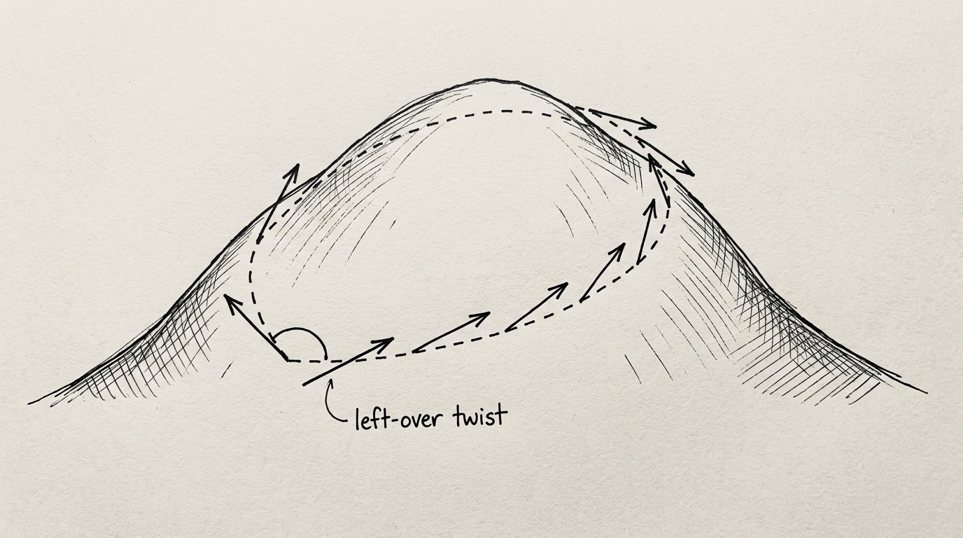
Take any small loop on the surface — say, the triangles surrounding one vertex — and parallel-
transport a vector all the way around it back to where it started. On a flat region, it comes back
pointing the same way it left. Where it doesn't, that mismatch angle (the holonomy
of the loop) is exactly what a singularity is: a point where the field genuinely cannot be smooth,
and the size of the mismatch (quantized in units of 360°/N for an N-RoSy field) is the
singularity's index.
Crucially, this reframes "where are the singularities" as a direct, computable property of whatever connection you choose — not something that only emerges after the fact from smoothing. That's what makes the paper's core promise possible: choose the holonomy pattern you want (i.e. choose exactly which loops should have a mismatch, and how much), and solve for the connection that's globally smoothest subject to producing exactly that pattern.
One linear system, hard constraints, a global optimality guarantee
Because a connection is just one number per edge, and both "how smooth is it" (deviation from Levi-Civita) and "what's its holonomy around each loop" (the singularity constraint) are linear in those numbers, the whole problem reduces to a single sparse linear system — no iteration, no local relaxation, no risk of getting stuck in a bad local optimum the way iterative smoothing can. The paper proves the result is globally optimal in a precise sense: among every connection achieving the prescribed set of singularities, it's the one closest to Levi-Civita (i.e. the smoothest possible one consistent with your constraints).
Why this composes well with other design decisions
Because this paper's input is simply a list of desired (location, index) pairs, it composes naturally with any upstream decision about where those should go — including symmetry constraints (make the list symmetric under a chosen mirror map to get a bilaterally symmetric field) or feature-driven placement (put singularities at natural anatomical/mechanical joints rather than mid-panel). The linear solve itself doesn't care how the list was chosen.